A Complete Guide to Types of Machine Learning
📚 Table of Contents
Introduction
Imagine you want to teach a computer to recognize pictures of cats, predict tomorrow’s weather, or recommend movies you might like. How would you do it? The answer lies in machine learning – a way of teaching computers to learn from data instead of programming every single rule by hand.
But here’s an interesting question: not all learning is the same, right? When you learn to ride a bicycle, someone shows you how (with supervision). When you learn to recognize patterns in clouds, you do it on your own (without supervision). When you train a pet, you give treats for good behavior (rewards). Computers learn in similar ways!
Machine learning can be categorized in many different ways, but one of the most useful approaches is to classify algorithms based on how much supervision or guidance they need during training.
Think of it like teaching styles:
- Supervised Learning: Like learning with a teacher who gives you questions AND answers
- Unsupervised Learning: Like exploring on your own to discover patterns
- Semi-Supervised Learning: Like having a teacher for some lessons but exploring on your own for others
- Reinforcement Learning: Like learning through trial and error with rewards and consequences
Based on the amount of supervision required, we can divide machine learning into four main categories:
- Supervised Machine Learning – The model learns from labeled data
- Unsupervised Machine Learning – The model finds patterns in unlabeled data
- Semi-Supervised Machine Learning – A mix of labeled and unlabeled data
- Reinforcement Learning – An agent learns by performing actions and receiving rewards
Some of these categories also have important sub-types:
Supervised Learning includes:
- Regression
- Classification
Unsupervised Learning includes:
- Clustering
- Dimensionality Reduction
- Anomaly Detection
- Association Rule Learning
Let’s explore each type in detail, understanding not just what they are, but why we need them and what problems they solve.
Supervised Learning
The Problem We’re Trying to Solve
Imagine you’re a college counselor, and every year, 5,000 students graduate. Some get job placements, and some don’t. Now, you want to help current students understand their chances of getting placed. How do you do that?
You could try to guess based on gut feeling, but that wouldn’t be very accurate. You could try to write rules like “If IQ is above 100 AND CGPA is above 8.0, then placement = Yes,” but real-world relationships are much more complex than simple if-then rules. Writing thousands of rules for every possible combination would be impossible!
What’s the real problem here?
We have historical data showing inputs (student IQ and CGPA) and outputs (whether they got placed). We can see the relationship, but we don’t know the exact mathematical formula that connects them.
What’s the root cause?
Human brains are good at spotting patterns but terrible at calculating precise mathematical relationships from thousands of data points. We need a computer to analyze all this data and find the hidden mathematical relationship.
How did people solve this before machine learning?
They used statistical methods and manual analysis, which were slow, limited, and often inaccurate for complex patterns.
So, how can we solve this problem better?
This is where supervised machine learning comes in!
What is Supervised Learning?
Supervised machine learning is all about learning from data that has both inputs and corresponding outputs. Your goal is to figure out the relationship between the inputs and the outputs. Once this relationship is learned, you can use it to predict the output for new, unseen inputs.
Think of it like this: imagine you’re studying for a math test. Your teacher gives you practice problems (inputs) along with the correct answers (outputs). By studying these examples, you learn the rules and formulas. Later, when you see new problems on the actual test, you can apply what you learned to solve them.
Example: Student Placement Prediction
Let’s say you have data for 5,000 students. For each student, you have two pieces of input information:
- IQ (Intelligence Quotient): How intelligent the student is
- CGPA (Cumulative Grade Point Average): The student’s academic performance
And for each student, you also have the output information:
- Placement Status: Whether the student got placed in a job or not (a “Yes” or “No” answer)
Here’s how the data might look for a few students:
| IQ | CGPA | Placement Status |
|---|---|---|
| 87 | 7.1 | Yes |
| 111 | 8.9 | Yes |
| 75 | 6.3 | No |
| 95 | 7.8 | Yes |
| 68 | 5.9 | No |
In this scenario:
- Input Columns: IQ and CGPA – These are the factors that influence the outcome
- Output Column: Placement Status (Yes/No) – This is what you want to predict
How does the algorithm learn?
A supervised machine learning algorithm analyzes all 5,000 examples. It looks at the IQ values, CGPA values, and placement outcomes, searching for patterns. It tries to find a mathematical relationship (like an equation or a decision boundary) that best explains how IQ and CGPA together determine placement status.
Once trained, if you give the algorithm new input values – say, a student with an IQ of 73 and a CGPA of 7.3 – it can predict whether that student will likely get placed or not.
Why is it called “supervised”?
It’s called supervised because the algorithm learns under the “supervision” of known output labels. Just like a teacher supervises your learning by checking your answers, the algorithm uses the correct outputs to guide its learning process.
Supervised learning is by far the most common type of machine learning you’ll encounter in real-world applications – from email spam detection to medical diagnosis to self-driving cars.
Two Main Types of Supervised Learning
Now here’s an important question: What if the output you’re trying to predict is different in nature? What if instead of predicting “Yes/No,” you want to predict a specific number, like a salary amount?
This brings us to the two sub-types of supervised learning, which depend on the nature of the output you’re trying to predict.
Regression
The Problem:
Let’s go back to our student example. Instead of just knowing whether a student gets placed (Yes/No), imagine you want to predict something more specific: How much salary will they earn?
Now the challenge changes. You’re no longer predicting a simple category like “Yes” or “No.” You’re trying to predict a specific number – maybe 4.5 lakhs per year, or 6.2 lakhs, or 8.7 lakhs. These numbers can have infinite possibilities within a range.
What’s different here?
The output is now numerical and continuous. Instead of choosing between fixed categories, you’re predicting a value that can be anywhere on a number line.
What is Regression?
Regression problems occur in supervised learning when your output column contains numerical, continuous values. This means the prediction you’re trying to make is a number that can vary smoothly.
Example:
Let’s modify our student example. Your goal now is to predict the package size (the salary in lakhs per annum) a student will get after college.
| IQ | CGPA | Package Size (Lakhs) |
|---|---|---|
| 87 | 7.1 | 4.5 |
| 111 | 8.9 | 6.0 |
| 75 | 6.3 | 3.5 |
| 102 | 8.2 | 5.8 |
| 93 | 7.5 | 4.9 |
In this case, the output (Package Size) is a number. The algorithm will learn the mathematical relationship between IQ, CGPA, and salary. Then, when you input a new student’s IQ and CGPA, it will output a predicted salary – perhaps 5.2 lakhs.
Even though it’s still a supervised problem (because you have both inputs and outputs), the nature of the output makes it a regression problem.
Other examples of regression problems:
- Predicting house prices based on size, location, and age
- Predicting a person’s age from their photo
- Predicting tomorrow’s temperature
- Predicting how many products will sell next month
- Predicting a student’s exam score based on study hours
All of these involve predicting a numerical value – that’s the key identifier of regression.
Classification
The Problem:
Now let’s return to our original question: Will a student get placed (Yes) or not placed (No)?
Notice something different here? You’re not predicting a number that can be 4.5 or 6.2 or 8.7. You’re predicting one of two specific categories: “Yes” or “No.”
What’s the key difference?
The output is categorical instead of numerical. You’re putting things into distinct bins or categories, not measuring them on a continuous scale.
Why can’t we use regression here?
Think about it: if you tried to use a regression model to predict “Yes/No,” what numbers would you use? You might assign Yes=1 and No=0, but then the model might predict 0.7. What does 0.7 mean? Is that “mostly yes”? This doesn’t make logical sense for categorical decisions.
What is Classification?
Classification problems occur in supervised learning when your output column is categorical. This means the prediction you’re trying to make falls into distinct categories or labels, not a continuous number.
Example:
Our original student placement prediction problem is a perfect classification problem:
| IQ | CGPA | Placement Status |
|---|---|---|
| 87 | 7.1 | Yes |
| 111 | 8.9 | Yes |
| 75 | 6.3 | No |
| 95 | 7.8 | Yes |
| 68 | 5.9 | No |
Here, the output “Placement Status” is categorical – it’s either “Yes” or “No.” The algorithm learns to draw a decision boundary that separates the two classes.
Other common classification examples:
- Email Filtering: Is this email spam or not spam?
- Weather Prediction: Will it rain today or not rain today?
- Image Recognition: Is this image a dog, cat, or bird?
- Medical Diagnosis: Does this patient have disease A, B, or C?
- Loan Approval: Should we approve this loan or deny it?
Binary vs. Multi-class Classification:
- Binary Classification: Only two possible categories (Yes/No, Spam/Not Spam)
- Multi-class Classification: More than two categories (Dog/Cat/Bird, Disease A/B/C/D)
Summary: Regression vs. Classification
Here’s the simple rule to remember:
If your supervised learning problem has a numerical output → it’s a REGRESSION problem
If your supervised learning problem has a categorical output → it’s a CLASSIFICATION problem
Both are supervised learning (they both use labeled data with inputs and outputs), but the nature of what you’re predicting determines which type it is.
Unsupervised Learning
The Problem We’re Trying to Solve
Imagine you’re a teacher with 1,000 students, and you want to understand your class better. You have data on each student’s IQ and CGPA, but here’s the catch: you have no labels. You don’t know who’s likely to get placed, who’s struggling, or which students are similar to each other.
What’s the problem?
With supervised learning, we always had the “answers” (output labels) to guide us. But what if we don’t have answers? What if we just have a massive pile of data and we want to understand it better, find hidden structures, or discover patterns we didn’t even know existed?
Why is this a problem?
In the real world, labeled data is expensive and time-consuming to create. Imagine labeling millions of images, categorizing thousands of customer reviews, or manually grouping billions of transactions. It’s often impossible or too costly!
What did people do before?
People would manually explore data, create visualizations, and use their intuition to find patterns. This was slow, limited to small datasets, and often missed subtle patterns that humans couldn’t detect.
So how can we solve this better?
This is where unsupervised machine learning comes in!
What is Unsupervised Learning?
Unsupervised machine learning is fundamentally different from supervised learning because your dataset only has input data – there are no corresponding output labels. This means you cannot predict an output because you don’t have one to begin with.
So what do you do with unsupervised learning if you can’t make predictions?
Great question! Unsupervised learning is used for a variety of important tasks:
- Finding hidden patterns in data
- Discovering natural groupings among data points
- Reducing complexity to understand data better
- Detecting unusual or suspicious behavior
- Discovering relationships between different items
Let’s explore the four main types of unsupervised learning and understand what problems each one solves.
Clustering
The Problem:
Imagine you’re running an e-commerce website with 10 million customers. You want to understand your customers better so you can create targeted marketing campaigns. But here’s the challenge: you don’t have pre-defined categories for your customers. You don’t know how many different “types” of customers you have or what distinguishes them.
What’s the core issue?
You have tons of data (purchase history, browsing behavior, demographics), but no clear structure. You need to organize this chaos into meaningful groups, but you don’t know what those groups should be or how many there are.
Why can’t we do this manually?
With millions of data points and dozens of features per customer, it’s impossible for humans to visually identify patterns or manually sort customers into groups.
What is Clustering?
Clustering is a technique where the algorithm identifies natural groupings or “clusters” within your data. It tries to group similar data points together without any prior knowledge of what those groups should be.
Think of it like organizing a messy closet: you naturally group similar items together (all shirts in one section, all pants in another) even without someone telling you how to organize it.
Example: Grouping Students
Imagine you have student data with only their IQ and CGPA – no “Placement Status” column. If you plot this data on a graph with IQ on one axis and CGPA on the other, you might see something like this:
          CGPA
           ↑
        10 |     * *
         9 |   * * *
         8 |  * * * *    * *
         7 | * *        * * *
         6 |           * * *
         5 |          * *
           |________________→ IQ
              60  80  100  120
Even though you never told the computer how many groups exist or what defines each group, a clustering algorithm would analyze this data and discover that there are, for instance, three distinct clusters of students:
- Cluster 1: Students with high IQ and high CGPA (top-right)
- Cluster 2: Students with high IQ but low CGPA (bottom-right)
- Cluster 3: Students with low IQ but high CGPA (top-left)
The algorithm automatically forms these groups based on which students are most similar to each other. Once you have these clusters, you could manually assign meaningful labels (e.g., “High Achievers,” “Underperformers,” “Hard Workers”).
Real-world Application: E-commerce Customer Segmentation
An e-commerce website can use clustering to group customers based on their purchasing behavior:
- Cluster 1: Discount shoppers who only buy during sales
- Cluster 2: Loyal brand customers who buy premium products regularly
- Cluster 3: Window shoppers who browse but rarely buy
- Cluster 4: Impulse buyers who make frequent small purchases
Once these groups are identified, the company can tailor marketing strategies for each segment. Discount shoppers get sale notifications, loyal customers get early access to new products, and so on.
The Power of Clustering:
Clustering algorithms can work with very high-dimensional data (data with many input columns) where you cannot visually identify groups yourself. Even with 50 or 100 features per data point, clustering can find meaningful patterns.
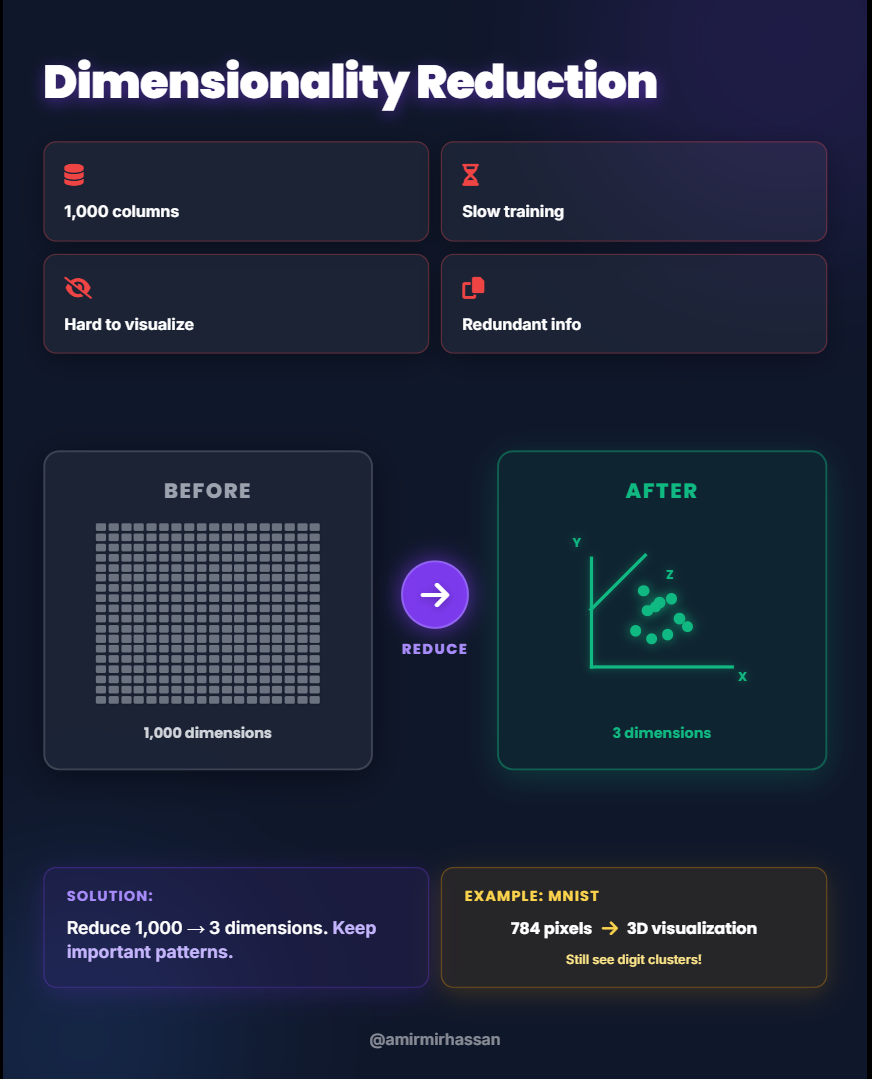
Dimensionality Reduction
The Problem:
Imagine you’re analyzing a dataset with 1,000 different columns (features). Maybe you’re studying genetic data with thousands of genes, or analyzing images where each pixel is a feature.
What’s the issue here?
Several serious problems arise:
- Computational Nightmare: Machine learning algorithms run extremely slowly with so many features. Training might take days or weeks instead of minutes.
- Storage Issues: Storing and processing huge amounts of data requires massive computing power and memory.
- Redundant Information: Many columns might be highly correlated or provide duplicate information. For example, if you have both “height in centimeters” and “height in inches,” one is redundant.
- Impossible to Visualize: Humans can only visualize 2 or 3 dimensions. You can’t plot or understand data with 1,000 dimensions.
- Curse of Dimensionality: With too many features, data points become so spread out that patterns become harder to detect.
Why is this a fundamental problem?
More features doesn’t always mean better learning. In fact, too many features can make patterns harder to find, not easier. It’s like trying to find a needle in a haystack – but the haystack keeps getting bigger!
What did people do before?
They would manually select which features to keep or remove, but this was guesswork and often threw away important information.
What is Dimensionality Reduction?
Dimensionality Reduction is a technique used to reduce the number of input columns (features) in your dataset while retaining as much important information as possible.
Think of it like packing for a trip: you can’t take your entire closet, so you pick the most versatile clothing items that let you create many different outfits with fewer pieces.
Example 1: House Features
Imagine a dataset for house prices where you have these input columns:
- “Number of Rooms” = 5
- “Number of Washrooms” = 3
Now ask yourself: are these really two independent pieces of information? Not really! Houses with more rooms almost always have more washrooms. These two features are highly correlated.
A dimensionality reduction algorithm might realize that these two columns combined represent a single underlying concept: “House Size” or “Living Space Capacity”.
Instead of keeping two separate columns, it could create a single new feature that captures information from both:
- “House Size Score” = (Number of Rooms × 0.7) + (Number of Washrooms × 0.3) = 4.4
This process of combining multiple features into a smaller set of more meaningful features is called feature extraction.
Example 2: MNIST Dataset (Image Visualization)
The MNIST dataset consists of images of handwritten digits (0-9). Each image is 28×28 pixels.
Here’s the problem:
If you represent each pixel as an input feature, that means each image has:
28 × 28 = 784 input features!
It’s completely impossible to visualize data in 784 dimensions. How can you understand the relationships between different digits?
The solution:
Using a dimensionality reduction technique like PCA (Principal Component Analysis), you can reduce these 784 dimensions down to just 2 or 3 dimensions.
The magic is this: even after this massive reduction (from 784 to 3), the algorithm preserves the relationships between data points.
Here’s what happens:
Original: Each digit image → 784 features
After PCA: Each digit image → 3 features (X, Y, Z coordinates)
Now you can plot these in 3D space! When you do:
- All the “0” digits cluster together in one region
- All the “1” digits cluster in another region
- All the “2” digits form their own group
- And so on…
Even in this massively reduced 3D space, similar digits stay close to each other, allowing you to visualize the relationships that exist in the much higher-dimensional original data.
Why This Matters:
Dimensionality reduction allows you to:
- Speed up training by reducing computational load
- Improve model performance by removing noise and redundancy
- Visualize complex data in 2D or 3D plots
- Save storage space and memory
- Understand data better by identifying the most important features
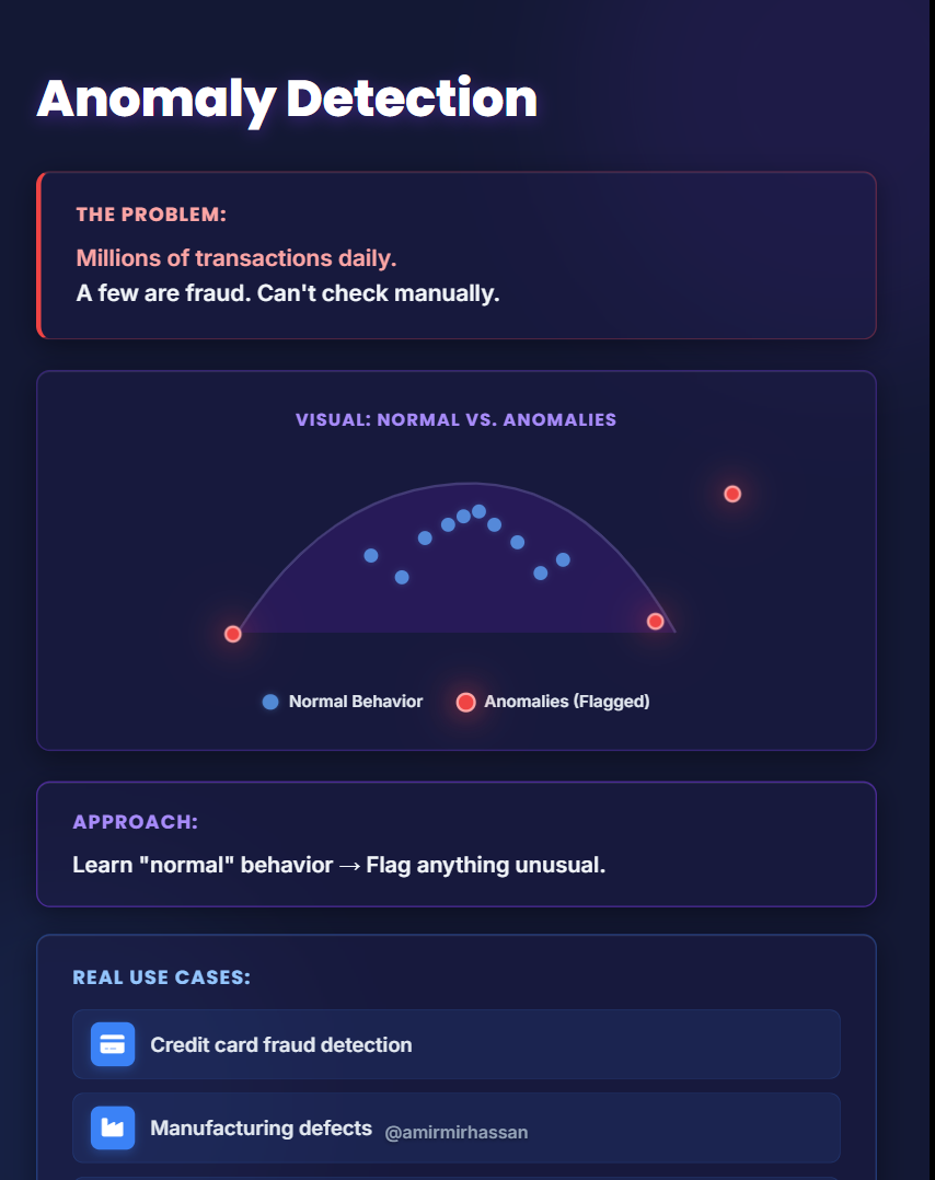
Anomaly Detection
The Problem:
Imagine you’re a bank processing millions of credit card transactions every day. Most transactions are normal – people buying groceries, paying bills, filling up gas. But hidden among these millions of normal transactions are a few fraudulent ones.
What’s the challenge?
- Fraudulent transactions are rare: Maybe only 0.01% of transactions are fraud. Finding them is like finding a needle in a haystack.
- Patterns constantly change: Fraudsters adapt their methods. What looked like fraud yesterday might look different today.
- You can’t label everything: You can’t manually review millions of transactions to mark which ones are fraud.
- False alarms are costly: If you block too many legitimate transactions, customers get angry. If you miss fraud, you lose money.
What’s the root cause?
Most of your data represents “normal” behavior. Fraud or defects are deviations from this normal pattern. You need to learn what “normal” looks like and then flag anything that doesn’t fit.
What is Anomaly Detection?
Anomaly Detection (also called Outlier Detection) is the process of identifying unusual patterns or “outliers” that deviate significantly from the norm. It’s crucial for detecting problems or fraudulent activities.
Think of it like a security guard at a building: they know what normal activity looks like (employees coming in the morning, deliveries at certain times). When something unusual happens (someone trying to enter at 3 AM, unusual package delivery), they pay attention.
How It Works:
- Training Phase: The algorithm learns from normal data. It builds a model of what “normal” looks like.
- Detection Phase: When new data comes in, the algorithm measures how far it is from “normal.” If it’s too far, it’s flagged as an anomaly.
Imagine a scatter plot:
Feature 2
              ↑
           10 |
            9 |   * * *
            8 |  * * * *
            7 | * * * * *
            6 |  * * * *
            5 |   * * *        ⚠
            4 |
           __|_____________________→ Feature 1
              1  2  3  4  5  6  7  8
Most points are clustered together (normal). The point marked with ⚠ is far from the main cluster – this would be flagged as an anomaly.
Real-World Examples:
1. Manufacturing Defects:
- Normal products have certain dimensions, weight, color
- Defective products deviate from these norms
- Anomaly detection flags defective items on assembly line
2. Credit Card Fraud:
- Normal: $50 grocery purchase in your home city
- Anomaly: $5,000 electronics purchase in a foreign country 2 hours later
- The system flags this as potentially fraudulent
3. Medical Diagnosis:
- Normal: Standard heart rate, blood pressure, test results
- Anomaly: Unusual combination of symptoms or test results
- Flags patients who need immediate attention
4. Network Security:
- Normal: Typical data traffic patterns
- Anomaly: Sudden spike in data transfer at odd hours
- Flags potential cyber attack or data breach
5. Predictive Maintenance:
- Normal: Machine vibrations, temperature, sound within expected ranges
- Anomaly: Unusual vibration pattern
- Predicts machine failure before it happens
Why This is Unsupervised:
Notice that during training, you don’t have labels saying “this is normal” and “this is an anomaly.” You just feed the system examples of normal data, and it learns to recognize what normal looks like. Then anything significantly different gets flagged automatically.
Association Rule Learning
The Problem:
Imagine you own a large supermarket with 50,000 different products. You need to decide:
- Which products should be placed near each other?
- Which products should be promoted together?
- What bundles or combinations should you offer?
What’s the challenge?
- Too many combinations: With 50,000 products, there are billions of possible pairs and combinations. You can’t manually analyze them all.
- Hidden patterns: Some relationships are obvious (bread and butter), but others are completely unexpected and impossible to guess.
- Need data-driven decisions: You can’t rely on intuition alone. You need to analyze actual purchase behavior.
What’s the root cause?
Customers don’t buy products in isolation – they buy combinations. Understanding these combinations can dramatically increase sales, but these patterns are hidden in millions of transactions.
What is Association Rule Learning?
Association Rule Learning aims to discover interesting relationships or “rules” between different items in large datasets. It answers the question: “If a customer buys item A, what else are they likely to buy?”
Think of it as discovering hidden connections: If you see someone buying a cake, they’re also likely buying candles. If someone buys a new phone, they’re likely buying a phone case.
How It Works: Market Basket Analysis
The algorithm scans through thousands or millions of shopping transactions (receipts) looking for patterns. It identifies rules like:
- Rule 1: {Bread} → {Butter} (If bread is bought, butter is often bought too)
- Rule 2: {Laptop} → {Laptop Bag, Mouse} (If laptop is bought, accessories follow)
- Rule 3: {Baby Diapers} → {Baby Wipes, Baby Formula}
Example: Supermarket Product Placement
Think about how products are arranged in a supermarket. They’re strategically placed to encourage purchases. How do supermarkets decide what goes next to what?
Step 1: Data Collection
They collect years of purchase history – every receipt, every transaction:
Receipt 1: Bread, Butter, Milk
Receipt 2: Bread, Butter, Eggs
Receipt 3: Bread, Jam
Receipt 4: Bread, Butter, Cheese
...
Receipt 100,000: Bread, Butter, Milk, Eggs
Step 2: Pattern Discovery
The algorithm analyzes this data:
- Total receipts scanned: 100,000
- Receipts containing Bread: 80,000 (80%)
- Of those 80,000, how many also contain Butter: 60,000 (75%)
Step 3: Rule Creation
Rule: {Bread} → {Butter}
- Support: 60% (60,000 out of 100,000 total receipts contain both)
- Confidence: 75% (75% of bread buyers also buy butter)
- Interpretation: If someone buys bread, there’s a 75% chance they’ll buy butter
Step 4: Action
The supermarket uses this insight:
- Place bread and butter close together
- Offer bundle discounts (bread + butter combo)
- If bread is on sale, place butter displays nearby
Famous Case Study: Beer and Diapers
Here’s one of the most famous examples of association rule learning in action:
A large retail chain (like Walmart) analyzed their transaction data and discovered something completely unexpected:
Discovery: {Baby Diapers} → {Beer}
Customers who bought baby diapers were also frequently buying beer – two products that seem completely unrelated!
The Theory:
After investigating, they developed a hypothesis: new fathers, sent to the store late at night to pick up diapers for their baby, would also grab a six-pack of beer for themselves.
The Action:
The store tested placing baby diapers near beer (even though this seems bizarre). The result? Sales of both products increased significantly!
This example beautifully illustrates how machine learning can uncover hidden patterns in data that humans might never intuitively discover, leading to significant business benefits.
Other Applications:
1. E-commerce Recommendations:
- “Customers who bought this item also bought…”
- Amazon’s recommendation engine uses association rules
2. Healthcare:
- Discovering which symptoms often occur together
- Understanding drug interactions and side effects
3. Content Streaming:
- “People who watched this show also watched…”
- Netflix and YouTube recommendations
4. Cross-Selling in Banking:
- Customers with checking accounts often need credit cards
- Home loan customers often need insurance
Association rule learning helps businesses understand their customers’ behavior patterns and make data-driven decisions about product placement, marketing, and recommendations.
Semi-Supervised Learning
The Problem We’re Trying to Solve
Imagine you work at Google Photos, and you need to build a system that can identify and label people in millions of photos.
Here’s the challenge:
- You have 100 million photos uploaded by users
- To train a supervised learning model, you’d need to manually label every single photo: “This is Dad,” “This is Mom,” “This is my friend John”
- Problem: Hiring people to label 100 million photos would cost millions of dollars and take years!
But wait, there’s another observation:
- Out of 100 million photos, maybe you only have labeled data for 100,000 photos (0.1%)
- The remaining 99.9 million photos are unlabeled (no one has told you who’s in them)
The Core Issue:
Getting labeled data is extremely expensive and time-consuming because it requires human effort:
- Someone manually looking at images to identify objects
- Someone listening to audio to transcribe speech
- Someone reading documents to categorize them
- Someone analyzing medical scans to diagnose diseases
But getting unlabeled data is cheap – people upload millions of photos, videos, and documents every day!
The Question:
Can we use the small amount of labeled data we have to help us learn from the massive amount of unlabeled data?
What is Semi-Supervised Learning?
Semi-supervised learning is a hybrid approach that sits between supervised and unsupervised learning. It’s used when you have:
- A small amount of labeled data (expensive, manually created)
- A large amount of unlabeled data (cheap, readily available)
The core idea is to use the small amount of labeled data to “bootstrap” or guide the learning process on the much larger unlabeled dataset. This helps improve the model’s performance without having to label everything.
Think of it like this: imagine you’re learning a new language. You have a few words with translations (labeled), but you also read tons of text without translations (unlabeled). You use your small dictionary to understand some words, then use context from the unlabeled text to learn new words.
How It Works:
Step 1: Use unsupervised learning (like clustering) on all the data to find natural groups
Step 2: Use the small amount of labeled data to label some of those groups
Step 3: The labels propagate to other unlabeled data points in the same group
Example: Google Photos Facial Recognition
Let’s walk through how Google Photos uses semi-supervised learning:
Scenario: You upload 1,000 photos of your family to Google Photos.
Step 1: Unsupervised Clustering (No labels yet)
Google Photos scans all 1,000 photos and identifies faces. Using facial recognition (an unsupervised technique), it groups similar faces together:
Cluster A: 250 photos of faces that look similar
Cluster B: 180 photos of faces that look similar
Cluster C: 200 photos of faces that look similar
Cluster D: 370 photos of various other faces
At this point, Google Photos doesn’t know who these people are – it just knows which faces look like the same person.
Step 2: Minimal Labeling (Supervision)
Google Photos shows you one photo from Cluster A and asks:
“Who is this person?”
You answer: “Dad”
That’s it! You only labeled one photo, not all 250.
Step 3: Label Propagation (Semi-Supervised Magic)
Google Photos takes your single label and applies it to all 250 photos in Cluster A:
- All photos in Cluster A are now automatically labeled “Dad”
You do the same for other clusters:
- One photo from Cluster B → You label it “Mom” → All 180 photos labeled “Mom”
- One photo from Cluster C → You label it “Sister” → All 200 photos labeled “Sister”
The Result:
Instead of labeling 1,000 photos manually (which would take hours), you only labeled 3 photos! The system used your tiny amount of supervision (3 labels) to automatically label hundreds of photos.
Why This is Powerful:
- Effort Saved: You labeled 3 photos instead of 1,000
- Accuracy: The clustering (unsupervised) already did good work grouping similar faces
- Scalability: This works even with millions of photos
- Best of Both Worlds: Combines the pattern-finding power of unsupervised learning with the accuracy guidance of supervised learning
Other Real-World Applications:
1. Speech Recognition:
- Labeled: 10 hours of audio with transcriptions (expensive)
- Unlabeled: 10,000 hours of audio without transcriptions (cheap)
- Use labeled data to guide learning from massive unlabeled dataset
2. Medical Imaging:
- Labeled: 1,000 X-rays diagnosed by doctors (expensive)
- Unlabeled: 100,000 X-rays without diagnoses (readily available)
- Use doctor diagnoses to help learn from all available images
3. Text Classification:
- Labeled: 500 news articles categorized by topic (manual work)
- Unlabeled: 500,000 news articles without categories (automatically collected)
- Use categories to learn patterns in massive text corpus
4. Fraud Detection:
- Labeled: 1,000 transactions marked as fraud/legitimate (investigated cases)
- Unlabeled: 10 million transactions without labels (daily operations)
- Use known cases to detect patterns in all transactions
The Key Takeaway:
Semi-supervised learning solves the labeled data bottleneck problem. It acknowledges that in the real world:
- Labeled data is valuable but scarce
- Unlabeled data is abundant but less useful alone
- Combining both gives you the best results with the least effort
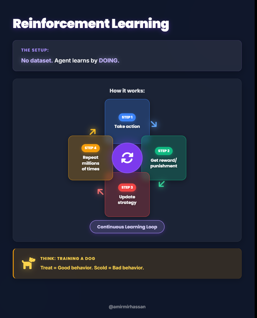
Reinforcement Learning
The Problem We’re Trying to Solve
Imagine you want to teach a robot to walk. How would you do it?
Can you use supervised learning?
Not really. You’d need to create a dataset like:
- Input: Robot’s current position, angle, joint positions
- Output: Exact movement commands for each joint
But here’s the problem: You don’t know the perfect movements yourself! You can’t create a labeled dataset because walking is too complex – it involves thousands of tiny decisions per second. Even human experts can’t write down the exact formula.
Can you use unsupervised learning?
No, because you’re not just trying to find patterns. You have a clear goal: make the robot walk forward without falling.
What’s the root cause of this problem?
For complex tasks like:
- Playing games (chess, Go, video games)
- Controlling robots
- Driving cars
- Managing stock portfolios
…there’s no fixed “dataset” to learn from. The environment is dynamic – it changes based on what you do. Every action leads to a new situation, and you need to figure out which actions lead to success.
How did nature solve this?
Think about how animals learn. A baby deer learns to walk not because its mother gave it a spreadsheet of “correct walking movements,” but through trial and error:
- The deer tries to stand (action)
- It falls down (consequence)
- It learns this approach doesn’t work
- It adjusts its approach
- Eventually, through many attempts, it learns to walk
Animals learn through rewards (finding food, avoiding pain) and punishments (hunger, injury).
What is Reinforcement Learning?
Reinforcement Learning (RL) is a unique type of machine learning where an algorithm (called an “agent”) learns to make decisions by interacting with an environment. The agent learns through a system of rewards and punishments.
Unlike supervised learning (no pre-existing dataset) and unlike unsupervised learning (there’s a clear goal), reinforcement learning is about learning through experience.
Analogy: Training a Pet
Think about training a dog:
- The dog does something (action) – maybe it sits
- If it’s good behavior, you give it a treat (reward)
- If it’s bad behavior, you might scold it (punishment)
- Over time, the dog learns: “When I sit on command, I get treats. When I jump on people, I get scolded.”
- The dog adjusts its behavior to maximize treats (rewards)
You don’t give the dog a manual or show it example videos. It learns through direct experience – trying things and seeing what happens.
Key Components of Reinforcement Learning
Let’s break down the building blocks:
1. Agent
- The learner or decision-maker
- Example: The robot trying to walk, the chess-playing program, the self-driving car AI
2. Environment
- The world the agent operates in
- Example: The road for a self-driving car, the chessboard, the physical world for a robot
3. State
- The current situation or configuration of the environment
- Example: Current positions of all chess pieces, current speed and position of a car, current joint angles of a robot
4. Action
- Choices the agent can make
- Example: Move chess piece, turn steering wheel left/right, move robot leg forward
5. Policy
- The agent’s strategy or “rulebook” that tells it what action to take in each state
- This is what the agent is learning!
- Example: “In this chess position, move the knight,” “When approaching a red light, slow down”
6. Reward
- A numerical signal given to the agent after an action
- Positive reward (good action): +10 points for reaching goal
- Negative reward / Punishment (bad action): -5 points for hitting a wall
- The agent’s goal: Maximize total reward over time
How the Learning Process Works
Let’s see a simple example with an agent in an environment:
Example: Agent Learning to Navigate
Imagine a simple environment:
- There’s fire (bad – gives negative reward)
- There’s water (good – gives positive reward)
- The agent can move left, right, up, or down
Environment:
[Water 💧]     [Empty]     [Empty]
[Empty]       [Agent 🤖]   [Empty]
[Empty]       [Empty]      [Fire 🔥]
The Learning Process:
Iteration 1:
- Agent observes the environment (sees fire, water, empty spaces)
- Agent has an initial policy (random or simple rules)
- Policy says: “Move right”
- Agent moves right
- Agent gets closer to fire → Receives negative reward: -5 points
- Agent learns: “Moving right in this situation is bad”
Iteration 2:
- Agent updates its policy based on the punishment
- New policy says: “Move left” (away from fire)
- Agent moves left
- Agent gets closer to water → Receives positive reward: +10 points
- Agent learns: “Moving left in this situation is good”
Iteration 3:
- Agent continues moving left
- Reaches water → Receives big positive reward: +100 points
- Agent learns: “Reaching water is the goal!”
Through thousands or millions of such iterations, the agent gradually learns the optimal policy – the best action to take in every possible state to maximize total rewards.
Real-World Application: AlphaGo
One of the most impressive demonstrations of reinforcement learning is AlphaGo, an AI program developed by DeepMind (owned by Google).
The Challenge:
Go is an ancient Chinese board game that’s far more complex than chess:
- Chess: About 10^120 possible game positions
- Go: About 10^170 possible positions (more than atoms in the universe!)
For decades, people believed it was impossible for AI to beat top human Go players because the game was too complex for traditional programming.
How AlphaGo Learned:
AlphaGo didn’t learn by studying books or watching human games (supervised learning). Instead, it used reinforcement learning:
- Self-Play: AlphaGo played millions of games against itself
- Reward System:
- Winning a game = Positive reward
- Losing a game = Negative reward / punishment
- Policy Improvement: After each game, it updated its policy (strategy) to make better moves
- Iteration: Played millions more games, constantly improving
The Results:
- 2016: AlphaGo defeated Lee Sedol, one of the world’s top Go players, 4 games to 1
- 2017: AlphaGo defeated Ke Jie, the world #1 ranked player at the time, 3-0
- During these matches, AlphaGo made moves that human experts had never seen before – creative, brilliant moves that changed how professionals think about Go
What Made This Special:
- AlphaGo learned strategies humans never discovered in 2,500 years of playing Go
- It learned entirely through self-play (reinforcement learning) without human guidance
- It demonstrated that RL can master tasks previously thought impossible for AI
Other Applications of Reinforcement Learning:
1. Robotics
- Teaching robots to grasp objects
- Training humanoid robots to walk
- Warehouse robots learning efficient routes
2. Game Playing
- OpenAI Five: Mastered Dota 2 (complex video game)
- DeepMind’s agents: Achieved superhuman performance in Atari games
3. Autonomous Vehicles
- Learning to drive in complex traffic
- Adapting to different road conditions
- Making split-second decisions
4. Finance
- Automated trading systems
- Portfolio optimization
- Risk management
5. Resource Management
- Data center cooling optimization (Google saved 40% on cooling costs)
- Energy grid management
- Traffic light optimization
6. Healthcare
- Personalized treatment recommendations
- Drug dosage optimization
- Medical device control
Why Reinforcement Learning is Challenging:
- No Fixed Dataset: The agent must generate its own data through exploration
- Delayed Rewards: Sometimes good actions don’t show benefits immediately
- Exploration vs. Exploitation: Should the agent try new things (explore) or stick with what it knows works (exploit)?
- Long Training Times: Agents might need millions of iterations to learn
- Reward Design: Defining the right reward function is crucial and difficult
Why It’s Powerful:
- Learns Autonomously: Doesn’t need labeled data or human examples
- Adapts to Change: Can adjust to new environments or situations
- Discovers Novel Strategies: Can find solutions humans never imagined
- Handles Complexity: Works in situations too complex for traditional programming
- Continuous Improvement: Can keep learning and improving over time
Summary: Understanding the Four Types of Machine Learning
Let’s recap the four main types of machine learning and when to use each:
Supervised Learning
When: You have input-output pairs (labeled data)
Goal: Predict outputs for new inputs
Types:
- Regression: Predicting numbers (salary, price, temperature)
- Classification: Predicting categories (spam/not spam, disease type)
Example: Predicting house prices based on size and location
Unsupervised Learning
When: You only have inputs (no labels)
Goal: Find hidden patterns and structure
Types:
- Clustering: Group similar items (customer segmentation)
- Dimensionality Reduction: Reduce features while keeping information
- Anomaly Detection: Find unusual patterns (fraud detection)
- Association Rules: Discover relationships (market basket analysis)
Example: Grouping customers by shopping behavior
Semi-Supervised Learning
When: You have lots of unlabeled data and a little labeled data
Goal: Use labels to guide learning from unlabeled data
Example: Labeling one photo per person, system labels thousands more
Reinforcement Learning
When: Agent must learn through trial and error in an environment
Goal: Learn optimal actions to maximize rewards
Example: Teaching AI to play games or control robots
Conclusion
Machine learning is not a single technique but a family of approaches, each designed to solve different types of problems. Understanding these types helps you choose the right tool for your specific challenge:
- Need predictions with labeled data? → Supervised Learning
- Want to discover hidden patterns? → Unsupervised Learning
- Have little labeled data but lots of unlabeled data? → Semi-Supervised Learning
- Need to learn through interaction and feedback? → Reinforcement Learning
The field of machine learning continues to evolve, with new techniques emerging and boundaries between categories blurring. But these fundamental types provide a solid foundation for understanding how machines learn and how we can apply these techniques to solve real-world problems.
As you continue your journey in machine learning, you’ll discover that many practical applications combine multiple types – using unsupervised learning for data exploration, supervised learning for prediction, and reinforcement learning for decision-making. The key is understanding the strengths and limitations of each approach so you can apply them effectively.